Evaluating performance in time-to-event data • ipeval

library(ipeval)
library(survival)

This vignette demonstrates how to estimate counterfactual performance metrics in right censored survival data.

Just like in the binary outcome, a IPT-weighted pseudopopulation is built which represents a situation in which everybody gets the treatment level of interest. On top of that, inverse probability of censoring weights are used such that the pseudopopulation also represents a situation where nobody gets censored.

Example 1, non informative censoring

We simulate some time-to-event data, where approximately half of patients get censored.

simulate_time_to_event <- function(n, constant_baseline_haz, LP) {
  u <- runif(n)
  -log(u) / (constant_baseline_haz * exp(LP))
}

simulate_data <- function(n, seed) {
  set.seed(seed)
  data <- data.frame(
    L1 = rnorm(n),
    L2 = rbinom(n, 1, 0.5),
    P1 = rnorm(n),
    P2 = rbinom(n, 1, 0.5)
  )
  data$A <- rbinom(n, 1, plogis(0.2 + 1.2*data$L1 - 0.3*data$L2))
  
  LP <- 0.8*data$L1 + 0.3*data$L2 + 0.5*data$P1 + 0.7*data$P2
  
  # time_0 is the uncensored untreated survival time,
  # time_1 is the uncensored treated   survival time 
  data$time_0 <- simulate_time_to_event(n, 0.04, LP)
  data$time_1 <- simulate_time_to_event(n, 0.04, LP - 0.5)
  
  # time_A is the uncensored survival time corresponding to assigned treatment 
  data$time_A <- ifelse(data$A == 1, data$time_1, data$time_0)
  
  # uninformative censoring
  data$censor_time <- simulate_time_to_event(n, 0.05, 0)
  
  # in practice, we only observe (time, status):
  data$status <- ifelse(data$time_A <= data$censor_time, TRUE, FALSE)
  data$time <- ifelse(data$status == TRUE,
                      data$time_A,
                      data$censor_time)
  return(data)
}

df_dev <- simulate_data(n = 10000, seed = 123)

summary(df_dev$time)
#>      Min.   1st Qu.    Median      Mean   3rd Qu.      Max. 
#> 5.110e-04 2.332e+00 6.108e+00 9.917e+00 1.333e+01 1.031e+02
summary(df_dev$status)
#>    Mode   FALSE    TRUE 
#> logical    5111    4889

Fit some models to validate:

model_naive <- coxph(
  formula = Surv(time, status) ~ P1 + P2 + A,
  data = df_dev
)

coefficients(model_naive)
#>        P1        P2         A 
#> 0.4123703 0.6248620 0.1643073

trt_model <- glm(A ~ L1 + L2, family = "binomial", data = df_dev)
propensity_score <- predict(trt_model, type = "response")

df_dev$iptw <- 1 / ifelse(df_dev$A == 1, propensity_score, 1 - propensity_score)

model_causal <- coxph(
  formula = Surv(time, status) ~ P1 + P2 + A,
  data = df_dev,
  weights = iptw
)

coefficients(model_causal)
#>         P1         P2          A 
#>  0.3993561  0.5819777 -0.4099308

The naive model estimates higher risk for treated patients than for untreated patients. The causal model correctly infers that treatment benefits patients. Note that the ‘true’ effect of $A$ was generated within a model that also conditions on $L1$ and $L2$ . Due to non-collapsibility, the estimated coefficient is not expected to coincide with the effect used in the data-generating mechanism.

We also simulate some validation data. In this example, we use the same data generating mechanism. We are interested in the predictive performance if every patient were to be assigned to treatment and remained uncensored, with a prediction horizon of 5 years.

df_val <- simulate_data(n = 10000, seed = 234)

To account for the time to event data, we specify a survival object as the outcome. As we have non-informative censoring in this example, we specify our censoring model to be estimated with Kaplan-Meier:

cfs <- ip_score(
  object = list("naive model" = model_naive, "causal model" = model_causal),
  data = df_val,
  outcome = Surv(time, status),
  treatment_formula = A ~ L1 + L2,
  treatment_of_interest = 1,
  time_horizon = 5,
  cens_model = "KM"
)
cfs
#> Estimation of the performance of the prediction model in a
#>  counterfactual (CF) dataset where everyone's treatment A was set to 1.
#> The following assumptions must be satisfied for correct inference:
#> - Conditional exchangeability requires that the inverse probability of
#>  treatment weights are sufficient to adjust for confounding between
#>  treatment and outcome.
#> - Conditional positivity (assess $ipt$weights for outliers)
#> - Consistency (including no interference)
#> - Correctly specified propensity model. Estimated treatment model is
#>  logit(A) = 0.21 + 1.19*L1 - 0.31*L2. See also $ipt$model
#> - Non-informative censoring. See also $ipc
#> 
#>         model   auc brier oeratio
#>    null model 0.500 0.176   1.000
#>   naive model 0.649 0.172   0.762
#>  causal model 0.649 0.167   0.952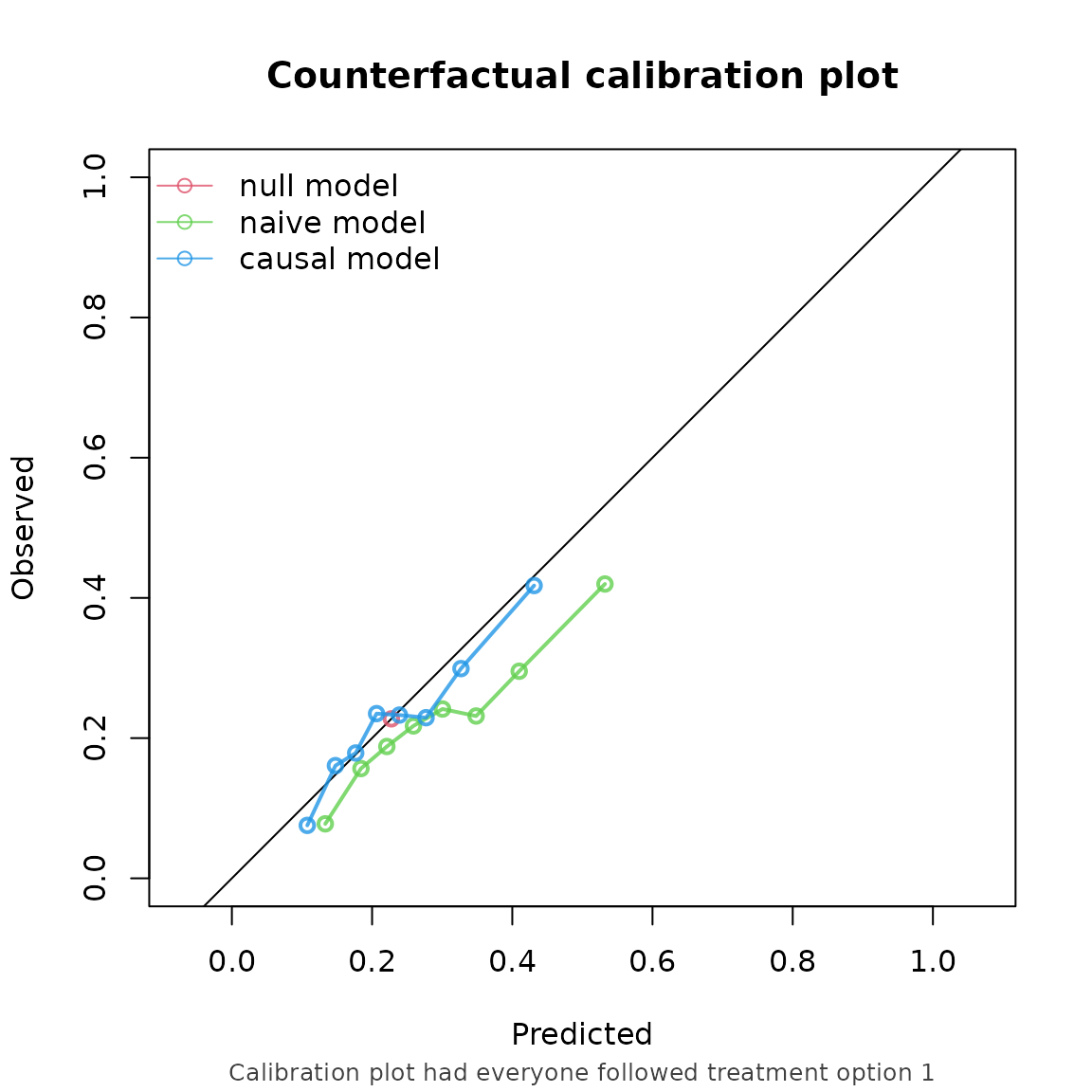

Example 2, informative censoring

We can also account for informative censoring. In this example, we keep the same prediction model as in example 1, but add an informative-censoring mechanism to the validation dataset.

df_val$censortime <- simulate_time_to_event(10000, 0.04, 0.1*df_val$L1 + 0.5*df_val$P2)
summary(df_val$censortime)
#>      Min.   1st Qu.    Median      Mean   3rd Qu.      Max. 
#> 1.696e-03 5.318e+00 1.312e+01 2.037e+01 2.739e+01 2.079e+02

df_val$status <- ifelse(df_val$time_A <= df_val$censortime, TRUE, FALSE)
df_val$time <- ifelse(df_val$status == TRUE,
                      df_val$time_A,
                      df_val$censortime)

summary(df_val$time)
#>      Min.   1st Qu.    Median      Mean   3rd Qu.      Max. 
#> 1.696e-03 2.324e+00 6.043e+00 1.064e+01 1.373e+01 1.665e+02
summary(df_val$status)
#>    Mode   FALSE    TRUE 
#> logical    5068    4932

We then set censoring model to “cox”, and supply the formula needed for the censoring model as the right hand side of cens_formula. Internally, the censoring distribution is estimated with this expression, from which the inverse probability of censoring weights are computed.

ip_score(
  object = list("naive model" = model_naive, "causal model" = model_causal),
  data = df_val,
  outcome = Surv(time, status),
  treatment_formula = A ~ L1 + L2,
  treatment_of_interest = 1,
  time_horizon = 5,
  cens_model = "cox",
  cens_formula = ~ L1 + P2,
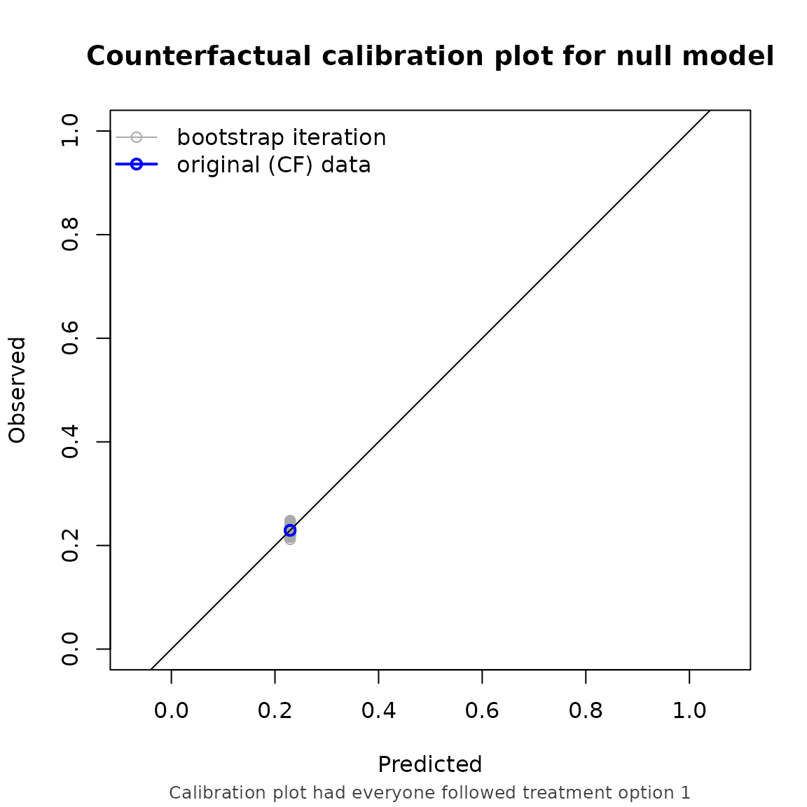
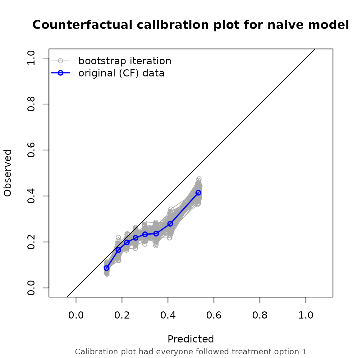
  bootstrap = 100,
  bootstrap_progress = FALSE
)
#> Estimation of the performance of the prediction model in a
#>  counterfactual (CF) dataset where everyone's treatment A was set to 1.
#> The following assumptions must be satisfied for correct inference:
#> - Conditional exchangeability requires that the inverse probability of
#>  treatment weights are sufficient to adjust for confounding between
#>  treatment and outcome.
#> - Conditional positivity (assess $ipt$weights for outliers)
#> - Consistency (including no interference)
#> - Correctly specified propensity model. Estimated treatment model is
#>  logit(A) = 0.21 + 1.19*L1 - 0.31*L2. See also $ipt$model
#> - Correctly specified censoring model. Estimated censoring distribution
#>  is P(C > t) = C_0(t)^exp(0.09*L1 + 0.52*P2). See also $ipc
#> 
#> auc
#> 
#>         model   auc lower upper
#>    null model 0.500 0.500 0.500
#>   naive model 0.635 0.616 0.655
#>  causal model 0.635 0.616 0.655
#> 
#> brier
#> 
#>         model brier lower upper
#>    null model 0.177 0.170 0.184
#>   naive model 0.175 0.169 0.180
#>  causal model 0.169 0.162 0.176
#> 
#> oeratio
#> 
#>         model oeratio lower upper
#>    null model   1.000 0.946 1.057
#>   naive model   0.768 0.725 0.811
#>  causal model   0.959 0.905 1.012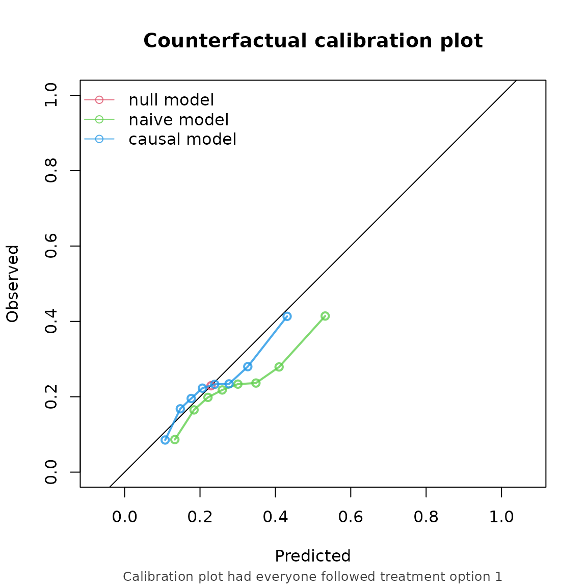

Note that the performance metrics we found in this example are approximately equal to the setting with non informative censoring. This is reassuring, as we correctly adjust for the informative censoring mechanism in this setting.