Generating longitudinal data with time-dependent confounding and fitting Marginal Structural Cox Models
Source:vignettes/longitudinal-data-and-cox-models.Rmd
longitudinal-data-and-cox-models.RmdThis vignette shows how to simulate longitudinal data with time-dependent confounding, fit a marginal structural Cox model (MSM), and obtain risk estimates under longitudinal treatment strategies. The resulting evaluation data and predictions are used in the next vignette.
The data-generating mechanism is adapted from Keogh and Van Geloven (2024) and follows the causal structure shown below.
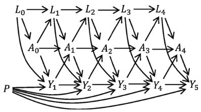
We generate repeated measurements of a time-varying confounder L and treatment A at five visits. At each visit, treatment depends on the current value of L and on the treatment at the previous visit. Both L and A also relate to the outcome, creating time-dependent confounding between A and outcome.
Outcome (event) and censoring times are simulated within each visit interval using the current values of A and L. If an event occurs before the next visit, the subject’s follow-up ends. Otherwise, new values of A and L are generated at the next visit and the process continues. This approach relies on the memoryless property of the exponential distribution.
simulate_longitudinal_data <- function(n, n_visits = 5, visit_times = 0:4, seed) {
  set.seed(seed)

  L <- matrix(nrow = n, ncol = n_visits)
  A <- matrix(nrow = n, ncol = n_visits)
  P <- runif(n)
  time <- rep(NA, n)
  status <- rep(NA, n)

  for (i in 1:n_visits) {

    # simulate A, L, even if a patient already has had an event (and therefore
    # misses subsequent visits). These are set to NA later.

    L[, i] <- if (i == 1) {
      rnorm(n, 0, 1)
    } else {
      rnorm(n, 0.8 * L[, i - 1] - A[, i - 1] + 0.1 * (i-1))
    }

    A[, i] <- if (i == 1) {
      rbinom(n, 1, plogis(0.5 * L[, i]))
    } else {
      rbinom(n, 1, plogis(0.5 * L[, i] + 0.8 * A[, i - 1]))
    }

    # To simulate outcome data (survival times and status) with these time varying variables, we simulate a
    # survival time at the first visit, using the corresponding values of A and L
    # at that visit. If subject survived until the next visit, we simulate
    # another survival time, this time using the new values of A and L, etc until
    # there is an event before the next visit. After the last visit, we just take
    # the last simulated survival time.
    new_event_time <- rexp(n, exp(-2 + -0.5 * A[, i] + 0.5 * L[, i] + 0.5 * P))
    new_censor_time <- rexp(n, exp(-3))

    if (i != n_visits) {
      time_until_next_visit <- visit_times[i+1] - visit_times[i]
    } else {
      time_until_next_visit <- Inf
    }

    new_time <- pmin(new_event_time, new_censor_time)
    new_status <- new_event_time < new_censor_time

    # if there was an event before the next visit, use that, if not, time and
    # status are kept at NA and are given another chance next iteration
    status <- ifelse(
      is.na(status) & new_time < time_until_next_visit,
      new_status,
      status
    )
    time <- ifelse(
      is.na(time) & new_time < time_until_next_visit,
      visit_times[i] + new_time,
      time
    )
  }

  # wipe A and L values after events (no visit after event)
  for (i in 1:n_visits) {
    A[, i] <- ifelse(time < visit_times[i], rep(NA, n), A[, i])
    L[, i] <- ifelse(time < visit_times[i], rep(NA, n), L[, i])
  }

  colnames(A) <- paste0("A", 0:(n_visits - 1))
  colnames(L) <- paste0("L", 0:(n_visits - 1))

  data.frame(id = 1:n, time, status, A, L, P)
}

df_dev <- simulate_longitudinal_data(20000, seed = 2)
df_val <- simulate_longitudinal_data(50000, seed = 3)
head(df_dev)
#>   id       time status A0 A1 A2 A3 A4         L0         L1         L2
#> 1  1  1.1809272   TRUE  0  1 NA NA NA  1.3404677  2.1378084         NA
#> 2  2 13.1015124   TRUE  1  0  1  0  0 -1.1157120 -1.5458058 -0.3413559
#> 3  3 37.3152659   TRUE  1  1  1  0  0  1.5065385  0.2223132 -0.6478227
#> 4  4  3.3843807   TRUE  0  0  0  1 NA -1.6099660 -0.8665974 -1.0083535
#> 5  5  0.7744242   TRUE  1 NA NA NA NA  0.9829932         NA         NA
#> 6  6 29.6789982  FALSE  1  1  1  0  1 -0.5279514 -0.7690418 -1.6548691
#>           L3         L4         P
#> 1         NA         NA 0.1848823
#> 2 -0.7969781 -0.8615738 0.7023740
#> 3 -3.4426019 -2.2972686 0.5733263
#> 4  1.1126904         NA 0.1680519
#> 5         NA         NA 0.9438393
#> 6 -1.9852403 -0.5948690 0.9434750
We now fit a marginal structural Cox model using inverse probability of treatment weighting (IPTW). Additional details can be found in the supplementary materials of Keogh and Van Geloven (2024).
We first convert the data to long format, with one row per visit per subject. The package provides helper functions for this transformation.
df_dev_long <- wide_to_long(
    df_dev,
    baseline_variables = c("id", "time", "status", "L0", "P"),
    wide_variables = list(A = paste0("A", 0:4),
                          L = paste0("L", 0:4)),
    visit_times = 0:4,
    outcome_times = df_dev$time
)

# set the time intervals correctly. The start time of the interval is given by
# visit_time. For the interval end time, use the start of the next interval, or
# the survival time, whichever happens earlier. If there is no next interval
# (last visit), use the survival time.
df_dev_long$time_end <- ifelse(
  df_dev_long$visit_time == 4,
  df_dev_long$time,
  pmin(df_dev_long$visit_time + 1, df_dev_long$time)
)
# We can use visit_time + 1 here because all visits are spaced 1 time apart

df_dev_long$status <- ifelse(
  df_dev_long$time_end == df_dev_long$time,
  df_dev_long$status,
  0
)
df_dev_long$time <- NULL

df_dev_long <- add_lag_terms(df_dev_long, "A", 1:4)
df_dev_long <- df_dev_long[, c("id", "visit_time", "time_end", "status", "L0", "P",
                "L", "A", paste0("A_lag_", 1:4))]
head(df_dev_long)
#>   id visit_time time_end status        L0         P          L A A_lag_1
#> 1  1          0 1.000000      0  1.340468 0.1848823  1.3404677 0       0
#> 2  1          1 1.180927      1  1.340468 0.1848823  2.1378084 1       0
#> 3  2          0 1.000000      0 -1.115712 0.7023740 -1.1157120 1       0
#> 4  2          1 2.000000      0 -1.115712 0.7023740 -1.5458058 0       1
#> 5  2          2 3.000000      0 -1.115712 0.7023740 -0.3413559 1       0
#> 6  2          3 4.000000      0 -1.115712 0.7023740 -0.7969781 0       1
#>   A_lag_2 A_lag_3 A_lag_4
#> 1       0       0       0
#> 2       0       0       0
#> 3       0       0       0
#> 4       0       0       0
#> 5       1       0       0
#> 6       0       1       0
To construct IPT weights, we model treatment assignment at each visit as a function of the confounder value at the current visit and the treatment value at the previous visit:
iptw_model <- glm(A ~ L + A_lag_1, family = "binomial", data = df_dev_long)
print(iptw_model)
#>
#> Call:  glm(formula = A ~ L + A_lag_1, family = "binomial", data = df_dev_long)
#>
#> Coefficients:
#> (Intercept)            L      A_lag_1
#>    -0.01636      0.49179      0.81078
#>
#> Degrees of Freedom: 71416 Total (i.e. Null);  71414 Residual
#> Null Deviance:       99000
#> Residual Deviance: 91790     AIC: 91800
The fitted coefficients are close to the true data generating coefficients. We then compute inverse probability of treatment weights and their cumulative products over follow-up:
iptw_propensity <- predict(iptw_model, type = "response")
iptw_prob_trt <- ifelse(
    df_dev_long$A == 1,
    iptw_propensity,
    1 - iptw_propensity
  )
df_dev_long$iptw <- 1 / iptw_prob_trt
df_dev_long$iptw_cumprod <- ave(df_dev_long$iptw, df_dev_long$id, FUN = cumprod)
summary(df_dev_long$iptw_cumprod)
#>     Min.  1st Qu.   Median     Mean  3rd Qu.     Max.
#>    1.149    2.302    4.710    9.884   11.118 1098.372
The cumulative IPT weights are used to fit the marginal structural Cox model:
cox_msm <- coxph(
  formula = Surv(visit_time, time_end, status) ~ A + A_lag_1 + A_lag_2 + A_lag_3 + A_lag_4 + L0 + P,
  data = df_dev_long,
  weights = iptw_cumprod,
  model = TRUE
)

print(cox_msm)
#> Call:
#> coxph(formula = Surv(visit_time, time_end, status) ~ A + A_lag_1 +
#>     A_lag_2 + A_lag_3 + A_lag_4 + L0 + P, data = df_dev_long,
#>     weights = iptw_cumprod, model = TRUE)
#>
#>              coef exp(coef)  se(coef) robust se       z        p
#> A       -0.394694  0.673886  0.004224  0.029613 -13.329  < 2e-16
#> A_lag_1 -0.400461  0.670011  0.004252  0.030549 -13.109  < 2e-16
#> A_lag_2 -0.303030  0.738577  0.004314  0.031234  -9.702  < 2e-16
#> A_lag_3 -0.214298  0.807108  0.004437  0.032816  -6.530 6.57e-11
#> A_lag_4 -0.181444  0.834065  0.004671  0.035575  -5.100 3.39e-07
#> L0       0.177327  1.194022  0.002152  0.015417  11.502  < 2e-16
#> P        0.356012  1.427624  0.007178  0.052135   6.829 8.57e-12
#>
#> Likelihood ratio test=32600  on 7 df, p=< 2.2e-16
#> n= 71417, number of events= 13326
We will now use cox_msm to estimate probabilities of
outcomes under interventions in our validation dataset. The
interventions of interest are ‘never treat’, where
is set to 0 at all visit times, and ‘always treat’, where
is set to 1 at all visit times. These treatment strategies are denoted
by
and
respectively.
For a given treatment strategy, the risk at time t can be obtained from the fitted MSM using the estimated cumulative hazard (see Equation e4, Keogh and Van Geloven, 2024, supplementary materials):
In practice, this can be done as follows for our evaluation dataset df_val:
compute_msm_probabilities <- function(model, data, treatment) {

  # get cumulative hazard fct from model
  bh <- survival::basehaz(model, centered = FALSE)
  cumhaz.fun <- stats::stepfun(bh$time, c(0, bh$hazard))

  # extract baseline covariates from data
  pred_under_int <- data[, c("id", "L0", "P")]

  # create a row for each visit
  pred_under_int <- pred_under_int[rep(1:nrow(data), rep(5, nrow(data))), ]
  pred_under_int$visit_time <- rep(0:4, nrow(data))
  pred_under_int$end_time <- pred_under_int$visit_time + 1

  pred_under_int$A <- treatment
  pred_under_int <- add_lag_terms(pred_under_int, "A", lag = 1:4)

  # compute the cumulative hazard contribution between each visit
  pred_under_int <- within(pred_under_int, {
    cumhaz_start <- cumhaz.fun(visit_time)
    cumhaz_end <- cumhaz.fun(end_time)
    lp <- predict(cox_msm, newdata = pred_under_int, type = "lp")
    contribution <- (cumhaz_end - cumhaz_start) * exp(lp)
  })

  # take the sum
  cumhaz <- tapply(pred_under_int$contribution, pred_under_int$id, FUN = sum)
  1 - exp(-cumhaz)
}

risk_under_0 <- compute_msm_probabilities(cox_msm, df_val, 0)
risk_under_1 <- compute_msm_probabilities(cox_msm, df_val, 1)

summary(risk_under_0)
#>    Min. 1st Qu.  Median    Mean 3rd Qu.    Max.
#>  0.3261  0.5321  0.5826  0.5832  0.6339  0.8743
summary(risk_under_1)
#>    Min. 1st Qu.  Median    Mean 3rd Qu.    Max.
#>  0.1391  0.2504  0.2822  0.2854  0.3170  0.5448
We will proceed with evaluating these predictions in the next vignette.