Counterfactual validation score

Usage

CFscore(
  object,
  data,
  outcome_formula,
  treatment_formula,
  treatment_of_interest,
  metrics = c("auc", "brier", "oeratio", "calplot"),
  time_horizon,
  cens.model = "cox",
  null.model = TRUE,
  stable_iptw = FALSE,
  bootstrap = 0,
  bootstrap_progress = TRUE,
  iptw,
  ipcw,
  quiet = FALSE
)

Arguments

object

One of the following three options to be validated:

a numeric vector, corresponding to risk predictions
a glm or coxph model
a (named) list, with one or more of the previous 2 options, for validating and comparing multiple models at once.

data

A data.frame containing at least the observed outcome, assigned treatment, and necessary confounders for the validation of object.

outcome_formula

A formula which identifies the outcome (left hand side). E.g. Y ~ 1 for binary and Surv(time, status) ~ 1 for time-to-event outcomes. In right censored data, the right hand side of the formula is used to estimate the inverse probability of censoring weights (IPCW) model. Alternatively, the IPCW can also be specified themselves using the ipcw argument, in which case the right hand side of this formula is ignored.

treatment_formula

A formula which identifies the treatment (left hand side). E.g. A ~ 1. The right hand side of the formula can be used to specify the confounders used to estimate the inverse probability of treatment weights (IPTW) model. E.g. A ~ L, where L is the confounder required to adjust for treatment. The IPTW can also be specified themselves using the iptw argument, in which case the right hand side of this formula is ignored.

treatment_of_interest

A treatment level for which the counterfactual perormance measures should be evaluated.

metrics

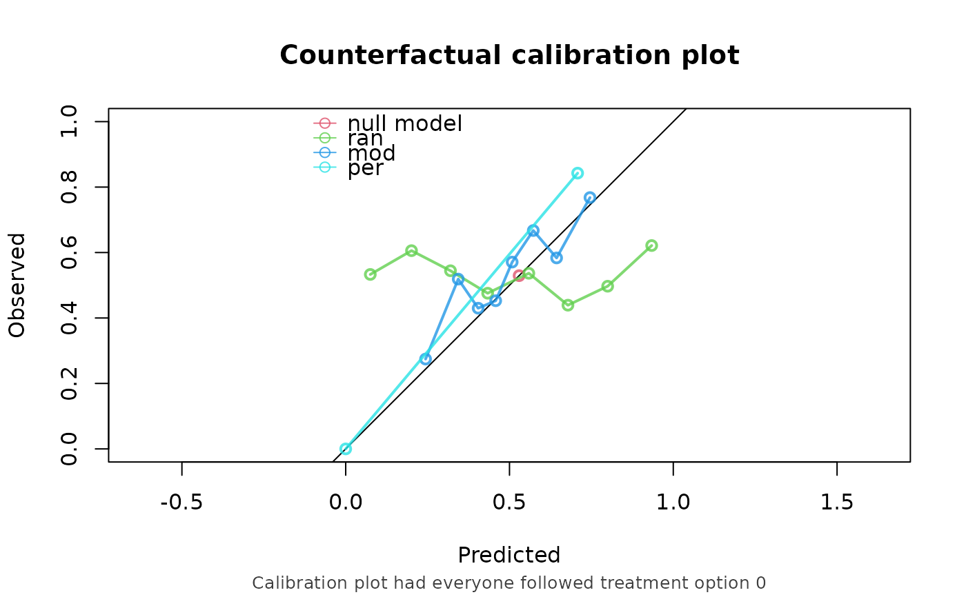
A character vector specifying which performance metrics to be computed. Options are c("auc", "brier", "oeratio", "calplot"). See details.

time_horizon

For time to event data, the prediction horizon of interest.

cens.model

Model for estimating inverse probability of censoring weights (IPCW). Methods currently implemented are Kaplan-Meier ("KM") or Cox ("cox") both applied to the censored times.

null.model

If TRUE fit a risk prediction model which ignores the covariates and predicts the same value for all subjects. The model is fitted using the data in which all subjects are counterfactually assigned the treatment of interest (using the IPTW, as estimated using the treatment_formula or as given by the iptw argument). For time-to-event outcomes, the subjects are also counterfactually uncensored (using the IPCW, as estimated using the outcome_formula, or as given by the ipcw argument).

stable_iptw

if TRUE, estimate stabilized IPTW weights. See details.

bootstrap

If this is an integer greater than 0, this indicates the number of bootstrap iterations, to compute 95% confidence intervals around the performance metrics.

iptw

A numeric vector, containing the inverse probability of treatment weights. These are normally computed using the treatment_formula, but they can be specified directly via this argument. If specified via this argument, bootstrap is not possible.

ipcw

A numeric vector, containing the inverse probability of censor weights. These are normally computed using the outcome_formula, but they can be specified directly via this argument. If specified via this argument, bootstrap is not possible.

quiet

If set to TRUE, don't print assumptions.

Value

A list with performance metrics.

Details

auc is area under the (ROC) curve, estimated ...

Brier score is defined as 1 / sum(iptw) sum(predictions_i - outcome_i)^2

oeratio represents the observed/expected ratio, where observed is the mean of the outcomes in the pseudopopulation. The expected is the mean of the predictions in the original observed population.

Examples

n <- 1000

data <- data.frame(L = rnorm(n), P = rnorm(n))
data$A <- rbinom(n, 1, plogis(data$L))
data$Y <- rbinom(n, 1, plogis(0.1 + 0.5*data$L + 0.7*data$P - 2*data$A))

random <- runif(n, 0, 1)
model <- glm(Y ~ A + P, data = data, family = "binomial")
naive_perfect <- data$Y

CFscore(
  object = list("ran" = random, "mod" = model, "per" = naive_perfect),
  data = data,
  outcome_formula = Y ~ 1,
  treatment_formula = A ~ L,
  treatment_of_interest = 0,
)
#> Estimation of the performance of the prediction model in a
#>  counterfactual (CF) dataset where everyone's treatment A was set to 0.
#> The following assumptions must be satisfied for correct inference:
#> - Conditional exchangeability requires that given IP-weights are
#>  sufficient to adjust for confounding and selection bias between
#>  treatment and outcome.
#> - Positivity (assess $ipt$weights for outliers)
#> - Consistency
#> - No interference
#> - Correctly specified propensity formula. Estimated treatment model is
#>  logit(A) = -0.08 + 0.95*L. See also $ipt$model
#> 
#>       model   auc brier oeratio
#>  null model 0.500 0.249    1.00
#>         ran 0.493 0.328    1.06
#>         mod 0.644 0.237    1.08
#>         per 1.000 0.000    1.50